scales, shards, and hash rings

how to distribute requests evenly and efficiently across servers.

How do you design an app to be scalable — elegantly adapt to 100 users, then 1000, then 100,000, and so on?

Vertical scaling means you upgrade your current server so it can handle the increased load. Two problems:

1. There are limits to how much CPU and RAM and whatnot you can add

2. Having one very powerful server still leaves you vulnerable in many ways. If rabid chimpanzees infiltrate your data center and start yanking cables (this is not a normal cause of failover, but you get the idea), your whole app will go down.

Horizontal scaling solves this problem by adding more servers and distributing your application’s load between those servers. Ideally, these servers are based in different parts of the world to minimize network latency and also the risk of a natural disaster or something taking down all your servers at once. Usually, users will connect to a load balancer which then evenly distributes the traffic between all the web servers.

It’s important that the servers are stateless (don’t have remember/store any client data between requests) so the load balancer can seamlessly redirect a client’s request to a different server if needed. In stateless architecture, requests from users can be sent to any web server, all of which fetch data from a shared data store. State data is either stored client-side (in the browser’s local storage) or a separate datastore. This is simpler, more robust, and scalable.

This figure shows how traffic moves through a horizontally scaled application.

In this essay I’m going to talk about a very specific problem: how to distribute requests evenly and efficiently across servers.

Let’s say we have s servers and x requests, each represented by a key.

Choosing the key is a design choice in and of itself. The key is any deterministic identifier that encourages affinity (same client/request type goes to the same backend), even distribution of requests between servers, and minimizes potential inefficiencies and conflicts.

For example, imagine you’re building a simple chat room. Chat messages for the same room must 1) arrive in correct order 2) access shared room state (e.g. who’s typing, unread counts)

This is most efficient when a room is handled by one server. You avoid having to sync state between servers every time anything happens + you can store things locally + message ordering is effortlessly preserved because they go through a single “queue” + you avoid race conditions that can happen when multiple servers access the same cache or datastore concurrently.

For all these reasons, room_id would be a good key. user_id, not so good.

Here are various use cases and the kind of key you might choose.

First, we hash each key. This will spread the keys (mostly) evenly across the hash space. The simplest way to distribute the keys mostly evenly would be a function like server = hash(key) % s.

But the whole point of doing this is that we might need to add more servers or disconnect a server. When s changes, every single request would need to be rerouted. Each server has its own cache (or slice of a cache) and its own local memory, both of which are tiers in which data is often stored for quick access.

When requests with a certain key are suddenly rerouted to a new server, cached data becomes irrelevant, leading to a lot of cache misses → needing to fetch data from slower datastores/services. So: the fewer keys are rerouted, the better. This is what consistent hashing accomplishes.

A hash ring is a data structure where you connect the tails of the hash space so the last possible value is before the first

Map servers onto the hash ring by hashing their ID or name or IP address. Map the keys onto the hash ring too.

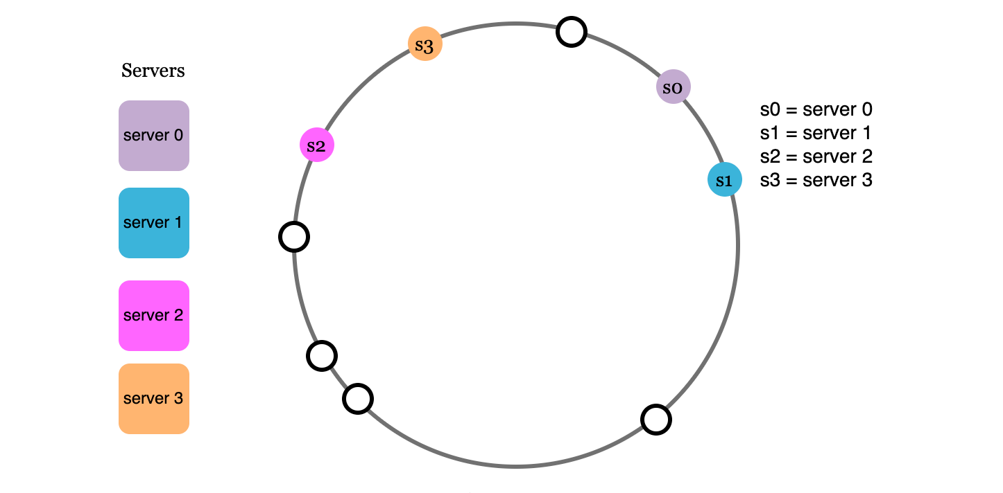
A key is simply stored on the first server after it on the hash ring. In the hash ring below, requests corresponding to key0 would be directed to server 0, key1 to s1; key2 to s2 and so on.¹

When a new server (s4) is added, instead of reassigning every key, we just reassign all the keys in the partition before the new server (between s3 and s4.)

When a server (s1) is removed, we just reassign all the keys in the partition before the defunct server (between s0 and s1.)

If you’re keen, you might have identified an issue. In these diagrams, the keys and servers are all evenly spaced, but we have no way of guaranteeing that. In fact, this scenario is much more likely:

We can fix this using virtual nodes - using V nodes to represent each server. leveraging the central limit theorem to reduce the variance of the spacing of the nodes. Basically: by artificially creating more nodes, we can make the distribution of the nodes — and therefore the partition size — more even.

You can also use more virtual nodes for more powerful servers, so that the load on each server (the total number of keys assigned to it) is proportional to its capacity.

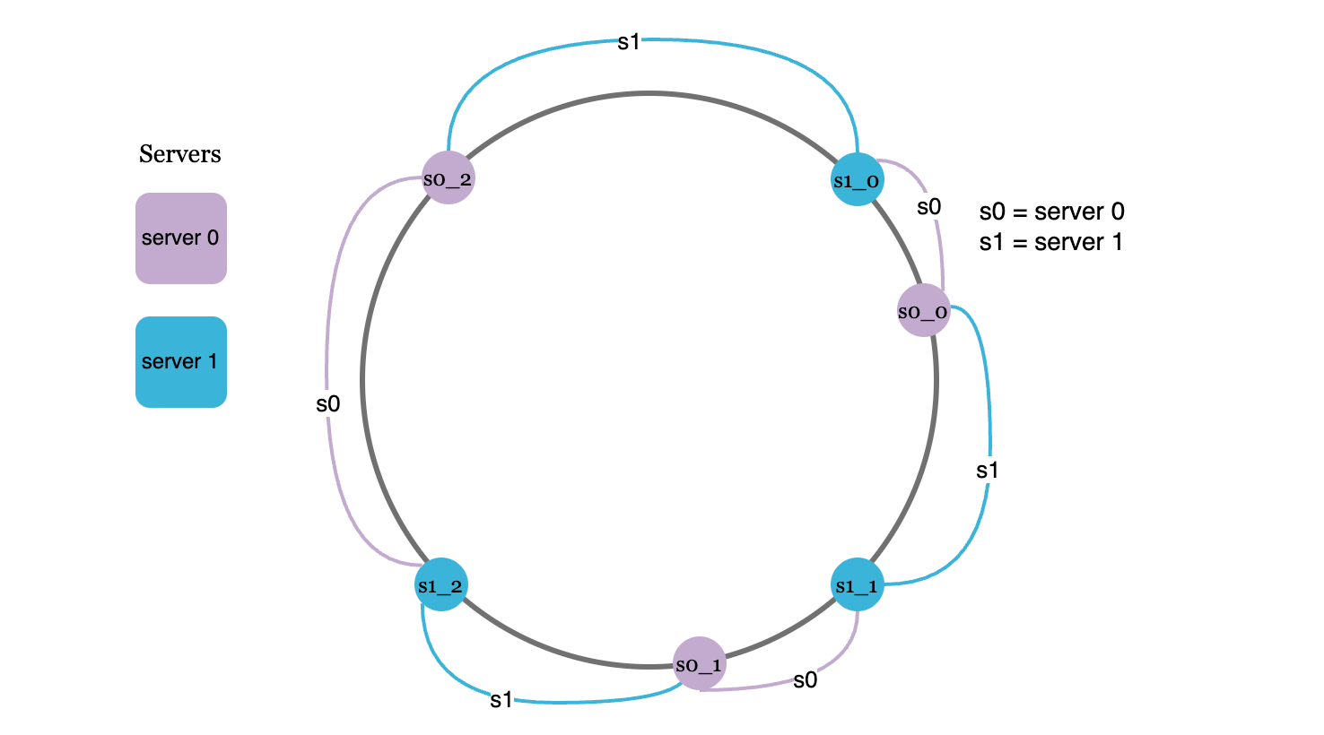
Here’s a diagram with two servers and 3 virtual nodes per server. Now, all the keys before s0_0, s0_1, and s0_2 are assigned to server 0. And so on, so forth for the other servers.

time complexity

The time complexity of looking up a key is O(log n) where n is the number of total nodes. Not the number of keys; the number of nodes.

This is done using binary search on an array of all the servers and virtual nodes on the hash ring.

Adding or removing a server has an average time complexity of O(V log n) where n is the number of existing nodes and there are V virtual nodes representing the new server.

You then have to remap all the keys, which takes O(k/s), where k is the number of keys and s is the number of servers. Effectively, remapping time increases linearly with the size of each partition.

data replication

Circular hashing is useful for partitioning all kinds of things between shards. Requests (as we talked about before) but also data.

It’s often useful to replicate data over servers to ensure high partition tolerance (system still works reasonably well even if one server goes offline).

Instead of a key being assigned to the next server on the hash ring, we assign it to the next N servers.

This introduces a new problem: data now also has to be synced across all replicas (imagine if the password for your email account was updated in all countries except Brazil).

We have to define two parameters:

1. a write quorum W: write operations must be acknowledged by W replica servers.

2. a read quorum R: read operations must wait for responses from at least R replica servers.

key0 is replicated on N=3 servers. if W is 1, the coordinator only needs one replica server to confirm “saved it” before it tells the client “write successful” if R is 2, the coordinator returns the data to the client after at least 2 servers confirm its value.

What if the replicas return different versions of the data? Usually, each value has a timestamp and the last write wins (LWW). In systems like Dynamo, it just returns all of the versions to the client and the client resolves the version conflict.

After the conflicts is resolved, the coordinator will perform read repair, asynchronously pushing the new value to the stale replicas.

We can tune the values of W, R, N to achieve the desired level of consistency.

• If W is low, writes are fast but you might accidentally write to an outdated server

• if R is low, reading is fast but you may get stale data

• if W is high, writing is slow and safe

• if R is high, reading is slow but accurate

If W + R > N, strong consistency is guaranteed. You can write something and be sure that the updates will be reflected consistently in all reads after the write is applied². This is because W + R > N ensures there must at least one node must have gotten both the write and the read. This system is reliable and consistent.

Otherwise, our system has eventual consistency, meaning it might take a bit for all the replica servers to get the update. This system is reliable and available. CAP theorem³ explains why consistency and availability are tradeoffs.

1. Images are taken from the ByteByteGo course on system design, which I highly recommend.

2. Strong consistency does not always mean that reads reflect live-time writes. It *does* mean that a client will not get an old value after another gets a fresh value. From the perspective of the clients, a write, once applied, is reflected in all future reads.

Imagine this: Client A successfully writes “X = 5”, acknowledged by nodes A, B, C, D. Immediately after, Client B reads from nodes D, E, F and returns X’s old value, 3.

Even with perfect versioning and timestamps, this could happen for multiple reasons: maybe D has acknowledged, but not fully applied, the write yet. Maybe D goes down temporarily. Either way, the write doesn’t have time to propagate.

Later, Client C reads X from A, D, F and gets 5.

This is still consistent because all clients see a sequence that makes sense: X = 3 → 5. No client ever sees X = 3 after seeing X = 5. That’s strong consistency, but not linearizability, because the writes and reads do not perfectly reflect the order in which they occurred.

3. In the ideal world, partition tolerance (reliability) is guaranteed, because network partition never occurs. Data written to s1 is automatically replicated to s2 and s3, so both consistency and availability are achieved.

But in the real world, network partition is always a possibility. We should never design a system that is not reliable.

Say s3 goes down and cannot communicate with s1 and s2. If clients can write data to s1 or s2, the system will still be available but the data will be inconsistent between the servers since s3 is unreachable. To keep the system consistent, we have to make writing unavailable to all servers.

For example, it is crucial for a bank systems to display accurate balance info. If inconsistency occurs due to a network partition, the bank system will return an error before the inconsistency is resolved. A social media platform or e-commerce site, on the other hand, will display an old version of a post instead of displaying nothing at all.